Real-Time Water Flow Simulation and Visualization

Clifford S. Champion
Supervised by Prof. Chris Anderson

January 2nd, 2006 – March 24th, 2006
UCLA Mathematics Directed Research (Math-199)

Abstract

The goal of this project was to develop a set of computer procedures that would computationally model the flow of water under various circumstances as well as to present to the user a sequence of images representing the water, all in real-time. The results of this project were two-fold. Firstly, a method for rendering 3-dimensional grid data to the computer screen was developed based on a method called “volumetric rendering using eye-aligned slices”. Secondly, the so-called “shallow water equations” were implemented and allowed for a real-time simulation of fluid flow within a cube-shaped container with a non-uniformly shaped bottom. Additionally, some experimentation took place in applying forces to the water simulation.

I. Volumetric Rendering

The first problem to be solved was that of how best to display a 3-d grid of data, let’s say a function f : N³→R, onto a computer screen using primitives supported by the GPU (usually triangles). This was our first task because it was uncertain whether or not such a visualization would be possible in real-time, let alone solving equations for water movement. One simple approach for visualizing f might be to simply render for each x in dom(f) a sphere or dot with a color representing its associated value in R; however, this visualization is very unsatisfactory for a number of reasons, especially if working with a coarse grid-size.

We then looked toward three other methods. Before discussing those methods it should be clear that when interfacing with a graphics processor unit (GPU), one is confined to rendering very simple objects such as points, lines, and triangles. So, more specifically, there is a need to develop a conversion scheme so that our function f can be visualized on the screen in terms of triangles.

The first two methods considered would have involved generating surfaces that bound 3-d regions of contiguous “mass” as determined by a threshold value c in range(f) and subsequently would have had to triangulate this surface into primitives that could be passed to the GPU. The third method, however, would involve visualizing f using “volumetric rendering” which would require no surface generation and no triangulation.

General volumetric rendering (using slices) works as follows. By exploiting a feature of modern GPU’s, we store our function f in the form of a 3-d texture and access its data through normalized (u,v,w) coordinates (a texture is just a finite, multi-dimensional array of RGBA color vectors and comes automatically with certain features such as filtering). Then we begin rendering our picture of f by calculating (u,v,w) coordinates of a planes that intersect dom(f) and use those coordinates to render cross-sections of f (called “slices”). In terms of GPU primitives, we simply setup two adjacent triangles forming a plane, and then we associate with these two triangles the calculated (u,v,w) values for each slice. Along the way we apply a mapping of our RGBA vectors to RGA values on screen; usually this is just an identity map or a simple scaling. This whole process then repeats, generating a desired number of slices. Lastly, each slice is rendered on top of one another with a certain degree of transparency so that the resulting image of f is such that we can “see inside of it”.

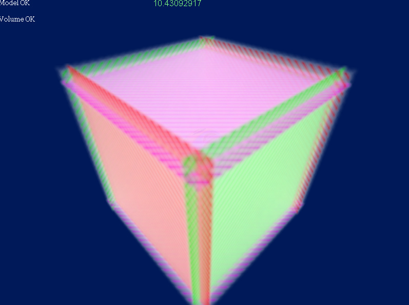
Additionally, we wanted renderings of our virtual scene to be perspective renders (non-orthographic), and we did not want to distinctly see our finite number of slices if we happen to rotate our camera around by 90 degrees. So the algorithm we implemented is a more specific kind of volumetric rendering called “volumetric rendering using eye-aligned slices” (not to be confused view-aligned slices). This method involves generating the set of planes such that their normal vectors are parallel with the view vector (the vector representing the orientation of the camera). In this case, the viewer can never rotate around to see a side of a slice because the slices are always “flat” to the camera. And with enough slices taken, the image becomes smooth in appearance, as pictured.

II. Shallow Water Equations

With a method for visualizing our function f completed, we could now move on to devising a scheme for generating realistic looking water flow. After some research and discussion, we decided to implement a model called the “shallow water equations” which is a derivation and simplification of the Navier-Stokes equations for fluid flow. This simplified model was chosen due to our design goal of wanting the simulation to run at real-time speeds, combined with initial testing that indicated solving the full Navier-Stokes equations in real-time may not have been feasible on today’s mainstream computers. Finding solutions to the Navier-Stokes equations involves finding a density function ρ(x,y,z,t) : N³xR→R; however, finding solutions to the shallow water equations involves finding a height function h(x,y,t) : N²xR→R which takes significantly less computation.

The first implementation we experimented with was solving for the height function h(x,t) : NxR→R using the shallow water equations in 2-d. The equations are

∂v/∂t + v·∂v/∂x + g·∂h/∂x = 0

∂(h-b)/∂t + ∂(v·(h-b))/∂x = 0

where b(x) is the height of the bottom, v(x,t) is the velocity in the x direction, and g is our gravitational constant. To numerically solve the system we used the Courant-Isaacson-Rees (CIR) method which includes finding characteristic coordinates and using an up-winding difference scheme. Performance in real-time turned out to be very good even before any optimizations were considered, providing and displaying a solution on a 120 point domain about 30 times per second (note that for purposes of visualizing, the solution in x was extended into y as constant). We then conducted experiments with applying forces of varying location, strength, and duration. Within certain bounds, the effects of these forces on the body of water were very pleasing and realistic in appearance.

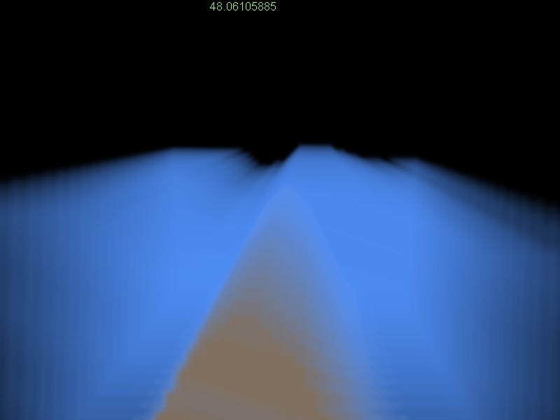
Building upon the encouraging results of the 2-d implementation, we moved forward to implement the shallow water equations in 3-d. The shallow water equations in 3-d are

∂v₁/∂t + v₁·∂v₁/∂x + v₂·∂v₁/∂y = -g·∂h/∂x

∂v₂/∂t + v₁·∂v₂/∂x + v₂·∂v₂/∂y = -g·∂h/∂y

∂(h-b)/∂t + div((h-b)·v) = 0

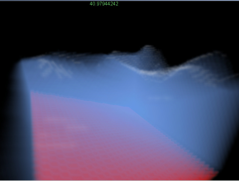
where v, h, and b are now defined on x and y and where v is a vector representing the velocity in the x and y directions (v1 and v2). After some research we chose a scheme for computing h in 3-d that would require minimal modification of the existing 2-d code and still provide the results we were looking for. We extended our current 2-d code by combining the CIR implementation with a method called “fractional steps”; basically it is applying our CIR method twice, once in the x direction for each y and once again in the y direction for each x. Much to our surprise, real-time performance was not significantly affected after migrating to 3-d. Our program still ran at real-time speeds, and computed and displayed a solution on a 72x72 point domain approximately 15 times per second.

Lastly, we again experimented with applying forces to our body of water and after some bug hunting saw some very exciting and satisfying results.

Conclusion

Much was accomplished in this project, both in developing a procedure for volumetric rendering and in implementing the shallow water equations for convincing simulations of water movement. What remains as a future endeavor is the integration of this water system with other physical systems, such as systems of rigid-body motion, to create a more entire simulation where objects can collide with the water and interact with it in a convincing manner. This would allow for some very interesting simulations.

Additional Information

Performance results cited in this report were based on our program running on the following computer specifications: Intel Pentium4 3.6Ghz, 1 GByte of dual channel DDR RAM, nVidia

GeForce Go 6800 PCI-Express, Microsoft DirectX 9.0c, Microsoft Windows XP Professional SP2. Our program was written in C++ and compiled in Microsoft Visual Studio .NET 2003 Standard Edition with compiler optimizations enabled for the SSE2 instruction set and most other compiler settings as their defaults. Code written for this project was integrated into an existing game engine framework (“Feather Engine V4”) written by Clifford S. Champion.